Guess-and-Check: The Breakfast of Statistical Champions

R-squared as a Measure of Model Fit

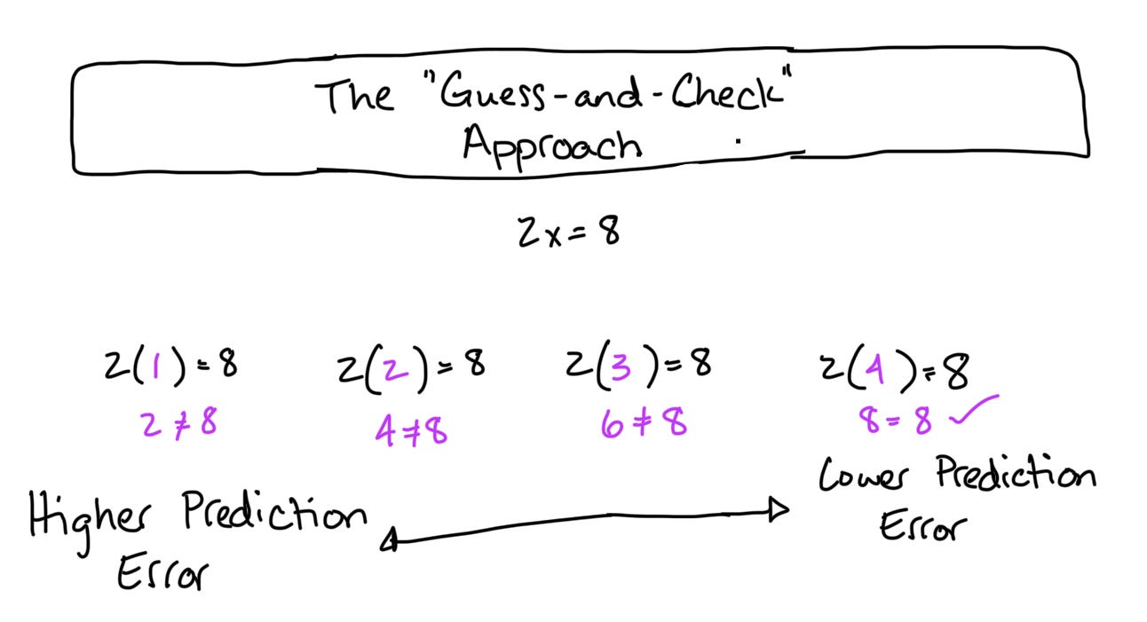
As a “math dumb” person, I was frequently encouraged to use the guess-and-check approach to solve algebra problems. I hated this method because it seemed less efficient than simply solving for x. While I was farting around “checking” many possible answers to a single problem, my classmates were finishing up their worksheets. When I learned there were computer tools that could solve these kinds of math problems, it felt like I’d won the lottery. Finally, something that’s smarter than me that can solve these problems more effectively. The crazy part? These computers solve the equations the exact same way that I was taught to.

If you’ve hung around statisticians for long enough, you’ve probably heard someone utter the phrase least squares estimation¹. This is a fancy way of saying that your computer guesses-and-checks possible solutions to a mathematical model. After each guess, it estimates the prediction error and compares it to the last solution. Was this new set of estimates better or worse? If the prediction error is lower, the computer keeps the current values and discards the old ones. If the prediction error is higher, the computer discards the current values and chooses a new set that’s different. The computer iterates like this until the prediction error is at its lowest value. The values with the lowest prediction error become the regression output that your statistical software provides.

My 8th grade self’s approach to algebra

R²: The Guess-and-Check of Statistical Software

Your statistical software’s guess-and-check approach is summarized by a single number called R². I’ve heard this alternatively referred to as:

• the coefficient of determination;

• the proportion of variance explained by your model;

• the sum squared error over the sum squared total; and

• a measure of the prediction error of your model.

You may be familiar with its daunting formula:

\(R^2= 1 - \frac{\sum_{i}^{n}{(y_i-\hat{y}_i})^2} {\sum_{i}^{n}{(y_i-\bar{y}})^2}\)

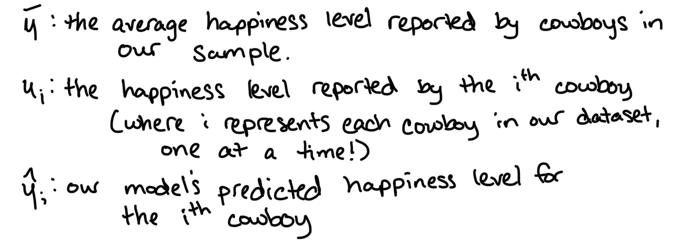
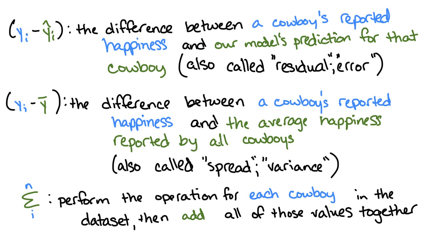
Sometimes, I’ll see this simplified using terms like SSE (sum squared error) and SST (sum squared total) or total variance and residual variance. Personally, I don’t find these simplifications helpful because they explain the fancy symbols by replacing them with other, less-fancy symbols. Instead, I’m going to walk through the formula using a simple model illustrating the relationship between a cowboy’s happiness and the number of horses he has²:

Some Helpful Notes

Symbol Bank

Parts of the Equation

What’s Next?

Now that we’re familiar with the R² formula, we can use it in the context of an actual statistical problem: we’ll use some archival data to determine whether there’s evidence of gender disparity among Marvel’s comic book heroes. So, dig out your cape and find the local phone booth! Until next time!

1. While the least squares estimator is one of the more common estimation strategies, it is by no means the only strategy. You may have heard of maximum likihood, Bayesian, or other estimators. These will almost certainly appear in a future post!

2. You can throw on your spurs and learn more about this hypothetical model in my last post on The Good, The Bad, and The Ugly.