

Variability is a fancy word researchers use to describe differences in the measurements they take from people. What I like most about this word is that it just makes sense. Let’s imagine that you and I were to share the name of our favorite album on the count of three. One… Two… Three… Did you say A by Jethro Tull? Probably not1, but the difference in our answers illustrates variability in the musical preferences of those who read this blog. Variability is a good thing to have in our data. Without it, we could not estimate a relationship between two variables! But just like the characters of a spaghetti western, variability can also be very, very bad. Think you’re ready to wrangle some relationships in your data? Well, saddle up and let’s git a wiggle on the three sources of variability you’ll find in your data.
The Good: Explained (Systematic) Variability
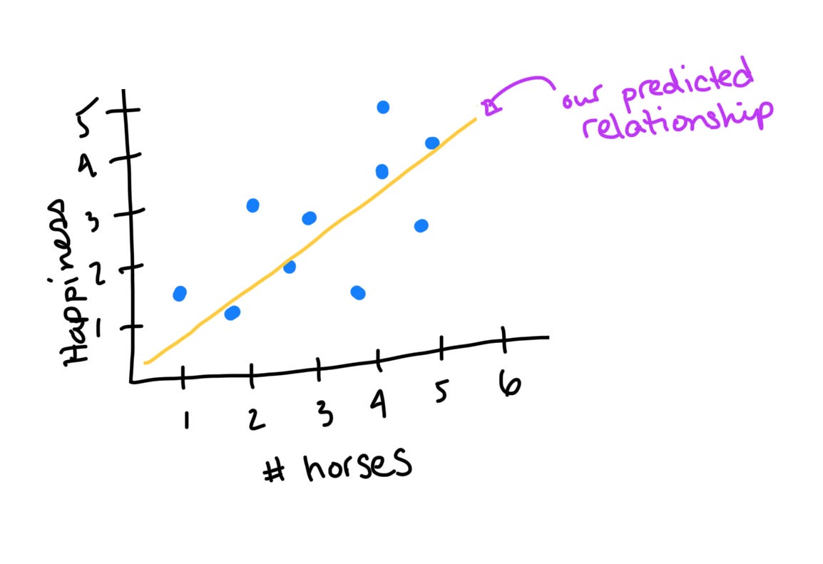
Let’s imagine that we want to empirically test old Waylon’s claim that cowboys are some of the lonliest and unhappy people in the world. To do this, I record my perception of each character in The Rifleman’s level of happiness on a scale from 1 (low) to 5 (high) alongside the number of horses they are said to have. Chances are, there’s some amount of variability in these measures: some cowboys have many horses and some have few; some cowboys are happy and others are not. We want to know whether those cowboys who have many horses are systematically happier than those who have few. If there is systematic variability, then there is a predictable relationship between horses and happiness - some amount of a cowboy’s happiness can be explained by the number of horses he has.
The Bad: Unexplained Variability from Nuisance Variables
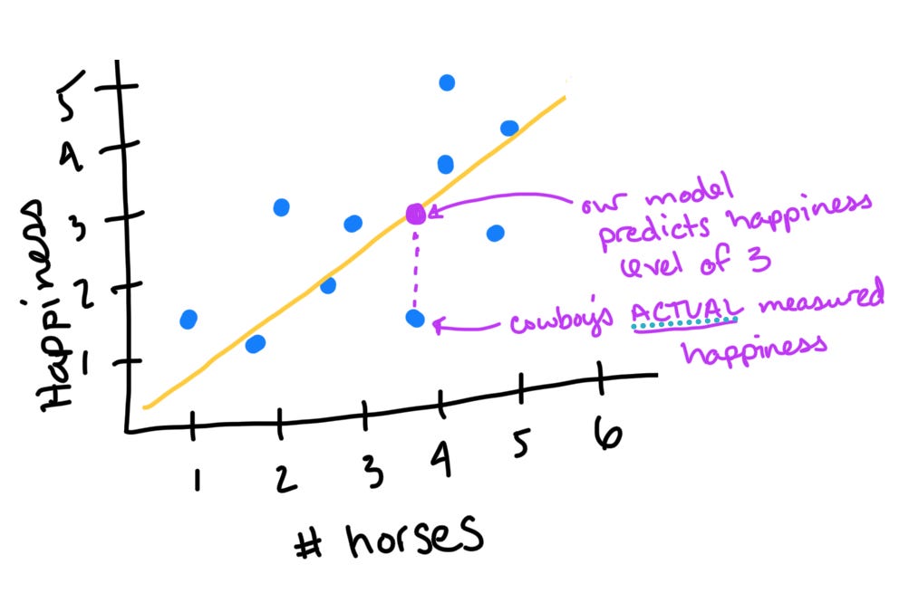
Of course, the relationship between horses and happiness is far from perfect and is affected by factors besides those we’ve captured in our model. Maybe a cowboy’s dog died. Maybe he lost his girl. These things would impact his happiness, but since we did not ask about them, we don’t know the extent to which they contribute. Instead, this unexplained variability contributes to the error of our model. This is a fancy way to say that our model cannot perfectly predict a cowboy’s happiness. This is illustrated by the difference between our prediction about a cowboy’s happiness and his actual happiness. For instance, here’s a cowboy who is feeling much worse than we would expect him to, given that he has around 4 horses:
Think of the many factors that impact your happiness on a day-to-day basis: how much sleep you’ve had, how hungry you are, what someone last said to you, whether you stubbed your toe… The variables we don’t measure are a nuisance (annoyance) to us because they reduce our model’s predictive power (maybe this is why we call them nuisance variables?). But they aren’t awful because we can still quantify them by reporting how well our model fits our data.
The Ugly: Unexplained Variability from Confounds
Sometimes, when we think we are modeling one thing, we are actually modeling another. For example, maybe cowboys who have many horses only have those horses because they are holding them for their friends. If this is true, then the number of horses that a cowboy has is a proxy measure of the number of friends he has. If we are aware that number of horses is a proxy for number of friends, then we can report this with our model and interpret it accordingly. But what happens when we don’t realize that we’ve collected a proxy measure? A confounding variable.
Confounding variables are particularly dangerous to mathematical models because we are often unaware of their presence. When we are unaware of confounds, we may draw inappropriate conclusions. Our model suggests that you could cheer a cowboy up by giving him a horse. Our discussion suggests that you should save the horse, find him a(nother) cowboy.
What’s Up Next?
Just because you’re working on the mathematical frontier, don’t treat your models like the Wild West! Think critically about your measures and whether they make sense, given the context. Consider alternative explanations for your results, and be transparent when reporting model accuracy through measures such as:
R2 and R2adj, simple measures of fit that use least squares estimation to determine how much of the outcome measure’s variability can be explained by the model’s parameters.
AIC and BIC, simple measures of fit that use maximum likelihood estimation to determine how likely our parameters are to have produced the outcomes we observed.
k-fold and leave-one-out cross-validation, which divide up our dataset to create a training set (to build the model) and test sets (to test the model’s predictive accuracy).
Next up, we’ll talk about measures of fit and demonstrate them using simple regression!
If you did, you get a double-plus-good bonus point! Unfortunately for you, this blog is like Who’s Line where everything is made up and the points don’t matter.