
An Unusual Beer Calls for Unusual Measures
An open-source dataset illustrates the strengths and weaknesses of various outlier exclusion methods, as well as their implications for out-of-sample prediction.

If you’ve taken a class from me or requested a statistical consultation, you’ve probably heard me lecture about the benefits of retaining outliers in a dataset. If we, as statisticians, are in the business of modeling truths in the world, then we need to be certain that our models predict a wide variety of out-of-sample observations. But sometimes, the unique qualities of an outlier justify its exclusion from a dataset. Here, I’ll walk through an example where this was the case.
The Dataset
The data I’ll be using to illustrate these points comes from an open-source dataset available on Kaggle.com, Beer Brewing Formulas and Recipes. This dataset contains detailed information about 25 different beers, including ingredient lists, brewing methods, and recommended food pairings. For this topic, I’ll focus on variables related to the composition of the beers, specifically:
abv
final_gravity (a measure of gravity/density after brewing)
ph (a measure of a beer’s acidity)
What Makes an Outlier?
Outliers can be described relative to their discrepancy, leverage, and influence.
By definition, any outlier represents a discrepancy - something about the observation is unusual relative to other data points. For illustration, let’s consider ABV and its relationship with pH level and final gravity (see Figure 1). Clearly, one beer’s ABV is not like the others…


The influence this beer has on our statistical predictions is determined by its leverage, or how unusual its combined values are within the context of the regression equation. In this case, this beer has an unusual ABV and final gravity but a completely unremarkable pH level. Therefore, it exerts little influence over the predictions generated by the pH level model and relatively more over those generated by the final gravity model (see left and right panels of Figure 3, respectively, for an illustration).


This occurs because discrepancies carry the same mathematical weight as any other observation within the context of least squares estimation (LSE), the error minimization approach associated with the General Linear Model. LSE operates like a tug-of-war with equally-matched opponents: discrepant observations that do not hold leverage will adjust the intercept of the model (i.e., shift the regression line upwards or downwards) while those that do hold leverage will adjust the slope of the model (i.e., shift the angle of the regression line).
While this difference may appear small visually, measures of model fit illustrate the outsized influence that a discrepant observation can have in some cases. Removing this beer from the dataset only changes the predictive power of our ph model by about 2% (high discrepancy + low leverage = low influence). By comparison, removing this beer changes the predictive power of our final gravity model by a whopping 62%1 (high discrepancy + high leverage = high influence)! With numbers like these, the choice seems clear: remove the outlier!
Method One: Remove the Outlier from the Dataset
Indeed, removing the outlier is a wise idea. A quick dig into the dataset reveals that the discrepant observation is The End of History. This beer was a publicity stunt (see Figure 2) and is considered the highest-ABV beer ever brewed. Because this observation represents a highly unusual beer (one that was controversial for its ABV and is unlikely to be replicated again), we are less likely to encounter beers like it out-of-sample. Therefore, I’m more willing to remove it from the dataset to improve model fit.

Although outlier removal is appropriate in this case, doing so does not solve our problem. Even after omitting The End of History, our model violates the assumptions of normality and homogeneity of variance (see Figure 4). Specifically, our model is less accurate in predicting the ABV of beers that have higher final gravity. This is illustrated most clearly in the right panel of Figure 4. Here, the dotted line at 0 represents the regression line, or the model’s best guess at a beer’s ABV based on its final gravity. The circles represent the observations in our dataset, and their vertical position relative to the line represents the direction and magnitude of our model’s error. For example, our model underestimates the ABV of observation #15 by about 4%. This tells us something important about the bounds of this model’s utility.


There is nothing inherently wrong with a model that systematically misrepresents some observations, provided these boundary conditions are communicated to readers:
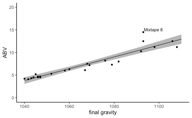
A visual inspection of the data revealed the dataset contained a novelty beer (The End of History) with an unusually high ABV (55%) that was brewed as a publicity stunt. Given this beer’s unusual nature and qualities, it was excluded from the dataset prior to analysis. A linear regression was used to model the relationship between final gravity and ABV among the remaining beers (n = 24). This analysis indicated that a beer’s final gravity is predictive of its ABV, B = 0.13, SE = 0.01, t = 12.81, p < .001. Namely, a 1% increase in a beer’s ABV is associated with an increase in final gravity of about 7.7 units. This relationship is reliable for most beers, although there are some notable exceptions (e.g., Mixtape 8 is a 14.5% ABV beer that our model underestimated as 10.7% ABV).
Method Two: Transform the Data to Linearity
The figures we’ve seen so far demonstrate an important quality of this dataset that provides a clue about the underlying nature of the relationship: ABV - and our model residuals - have a positive skew (see Figures 4 and 6). This makes sense - ABV is a proportion representing the amount of alcohol contained in a particular beverage relative to its overall volume. Therefore, ABV has both a hard floor (0) and a hard ceiling (100). Given that beers are alcoholic beverages, it makes sense that we would see a ceiling but not a floor effect; the particulars of beer brewing explain why the ceiling is much lower here than we might expect. Together, data and theory suggest there may be evidence for a non-linear relationship between final gravity and ABV. Although a full discussion on non-linear relationships is beyond the scope of this post, the information presented so far suggests that a log transformation will resolve the violation of assumptions.
While log transformation alone successfully improves the predictions of our model, it still fails to adequately capture the properties of The End of History. This is illustrated by plots of the residuals (see Figure 6) and by the widening error ribbons on the right-hand side of Figure 7, signifying that we are less confident in our model when predicting the ABV of beers with a higher final gravity.


Applying both approaches - removing the offending outlier *and* applying the appropriate transformation - results in a model that can explain 86% of the variance in ABV both within and out-of-sample (i.e., R-squared and adjusted R-squared, respectively). This model also appropriately captures the small but significant relationship between a beer’s final gravity and its ABV:
A visual inspection of the data revealed the dataset contained a novelty beer (The End of History) with an unusually high ABV (55%) that was brewed as a publicity stunt. Given this beer’s unusual nature and qualities, it was excluded from the dataset prior to analysis. Initial analyses consistently underestimated the ABV of beers with the highest final gravity, suggesting a non-linear relationship between the variables. Therefore, a linear regression was used to model the relationship between final gravity and log-transformed ABV among the remaining beers (n = 24). This analysis indicated that a beer’s final gravity is predictive of its log-transformed ABV, B = .02, SE = .001, t = 17.56, p < .001. Although the small standard error and large adjusted R-squared value (.93) indicate a great deal of confidence that this relationship will generalize out-of-sample, the magnitude of the relationship (a 1% increase in a beer’s ABV is associated with an increase in final gravity of about 50 units) calls into question the practical significance of this finding. Therefore, we encourage brewers and consumers to use caution when interpreting these findings.
Closing Thoughts
As statisticians, we have the important job of both analyzing and interpreting our data. It isn’t enough to perform formulaic analyses; accurately modeling truths about the world requires us to dig into a dataset and allow its unique qualities to inform our analytic decisions. I hope this post encourages you to think differently about outliers… and, perhaps, about beers in general!
Cheers!
Dr. V
These values were determined by comparing the R-squared values of each regression with and without the discrepant observation.