
Still No Superhero Bias!
Is There a Superhero Bias? Part III

After learning about some issues with the dataset I used for a previous post, I went ahead and performed the analyses a second time on the correct dataset. Spoiler alert: the results are nearly identical to what I observed before. Read on to learn about my process for analyzing the data in greater detail!
Cleaning the Data
Loading in the new file results in a dataset containing 16,376 cases and 13 variables. I’m planning to use the following for my analyses:
name: the character’s name, which serves as a unique ID for this dataset. Unlike a subject/case number, this variable de-anonymizes our dataset.
alignment: the character’s moral alignment (Bad, Good, Neutral).
gender: the character’s gender identity1 (female, male)
identity: whether the character’s identity is public (e.g., Tony Stark is Iron Man), secret (e.g., Bruce Wayne is secretly Batman), no dual identity (e.g., Thor), or known to authorities (e.g., Venom).
appearances: the number of times a character has appeared in Marvel’s comic books.
year: the year in which the character first appeared in Marvel’s comic books.
An initial inspection indicates that there are no duplicate cases in the data, although altered characters are mentioned more than once. For example, unique versions of Anthony Stark/Iron Man are represented by four cases in our dataset:
Anthony Stark (Skrull): an evil skrull shape-shifts into the form of Tony Stark.
Anthony Stark (Onslaught Reborn): a version of Tony Stark possessed by the villain, Onslaught.
Anthony Stark (Doppelganger): a doppelganger created by Magus and Anthropomorpho.
Anthony Stark (Counter-Earth): Stark as he exists in an alternate reality in which he never became Iron Man.
These characters are sufficiently different that I think it wise to count them as separate cases.
Several characters in the dataset are classified as genderfluid (n = 2) or agender (n = 45). I’ve removed these due to their under-representation and to improve the reliability of my model estimates. Interested readers are encouraged to analyze data from these characters as a unique subsample.
Exploring the Data
Descriptive statistics confirm the reported trend that the Marvel Universe contains more male characters - and gives them more page time - than characters of other genders.


Additionally, I can see that our key predictive variable (gender) is not correlated with other potential variables of interest. That is, I can’t predict a character’s alignment or the nature of their identity from their gender. Statistically speaking, we’d refer to this as data-driven multicollinearity.


‘Lude 1: Multicollinearity
Multicollinearity is a fancy word that means there are strong correlations between model predictors. This is problematic when our statistical goal is to make inferences2 about a population of interest, to use our statistical equation as a model of a phenomenon in the world. When the predictors of our model are strongly correlated, it becomes difficult to know which is responsible for driving the observed relationship with the outcome variable.
One non-mathematical example of this is my love of Samuel L. Jackson movies. Pulp Fiction, Inglourious Basterds, Django, Jurassic Park… if Samuel L. Jackson is in a movie, I will probably like it. Is this because I like Samuel L. Jackson’s acting? Or is it because all the Samuel L. Jackson movies in my sample are also action movies? For some of you, the solution to this problem is simple: watch a Samuel L. Jackson movie that is not an action movie, and see if you like it. If we’re experimentalists, we can easily implement this change in our study design3. But if we’re dealing with quasi-experimental or non-experimental data, tough noogies! We simply have to choose one of the predictors and move on. Fortunately, this isn’t the case with our dataset, so we can get back to…
Exploring the Data
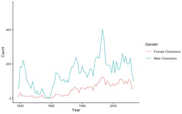
Counting the number of characters of each gender introduced by year shows that male characters’ introductions in the Marvel Universe are cyclic: large numbers were introduced in the early 1940s, 1960s, 1970s, and 1990s. In contrast, the number of female character introductions seems to be increasing over time.
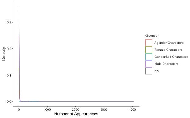
Another thing I notice is that the outcome variable of interest (number of appearances) is strongly skewed. This has implications for our analysis approach. General linear modeling approaches (e.g., linear regression, ANOVAs) assume that the model residuals (i.e., errors) will be normally distributed and homogenous. This is never the case when an outcome measure is skewed4.
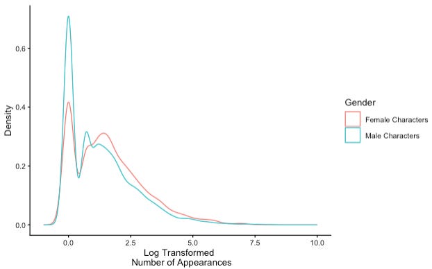
Log transforming the number of appearances dramatically reduces the skewness of the outcome variable, ensuring that the estimated marginal means (i.e., our calculations of the average number of appearances per group) are not dramatically affected by outlier characters who appear a disproportionate number of times relative to their peers4.
Stating Our Hypotheses
I want to test several hypotheses, informed by others’ work and my own curiosity:
H1: Male characters are over-represented in the Marvel Universe, relative to female characters (original hypothesis).
H2: Male characters’ over-representation in the Marvel Universe depends on the nature of their identity (e.g., maybe male characters are more likely to have public identities).
H3: Male characters are over-representation in the Marvel Universe depends on their alignment (e.g., maybe male characters are more likely to be good).
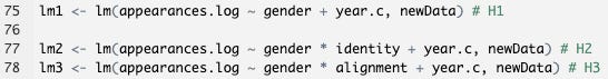
Each of these hypotheses must be tested with a different model:
H1: This model includes the main effect of gender and controls for changes over time by using year as a covariate.
H2: This full-factorial model includes gender and identity. It also controls for changes over time by using year as a covariate.
H3: This full-factorial model includes gender and alignment. It also controls for changes over time by using year as a covariate.
Building Our Models
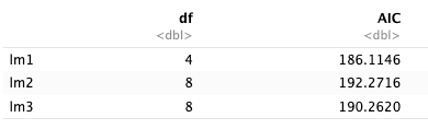
Rather than burn up statistical degrees of freedom by independently analyzing all three models, I can use AIC values5 to compare the models and determine which is most likely to have produced our data. This analysis indicates that the model associated with H1 is most likely to have produced our data.
Interpreting The Model
After removing 1,834 cases without a specified gender or appearance count6, I used linear regression to predict a Marvel character’s number of appearances from their gender, while controlling for year. Although the model provided better predictions than simply assuming every character appeared 18 times (the average number of appearances, back-transformed from the log scale), F(2, 13916) = 70.57, p < .001, gender and year could only explain 1% of the variance in characters’ number of appearances. On average, female characters appear one more time than their male counterparts7, B = 0.32, SE = 0.03, t = 11.67, p < .001. Although the results of this analysis strongly suggest that this result is replicable out-of-sample, the overall effect is small enough to be negligible, and we can conclude that on the whole, female characters appear just as often as male characters in the superhero franchise.
BUT THAT DEFIES ALL LOGIC!
Yes, the results of the analysis run contrary to the descriptive statistics from our data. But remember, we are not interested in concluding whether male characters have appeared more times than female characters in the Marvel Universe. We want to know whether we can predict a superhero’s gender based on their appearance record. Our answer (no!) can be explained by considering the density plot depicting number of appearances by gender.
In a density plot, the height of a line (y-axis) corresponds to the number of times that a specific value (x-axis) appears in a dataset. The general shape of our density plot illustrates several points:
many male characters make short appearances, as indicated by the high blue bump on the left side of the graph.
a small number of male characters appear many times, as indicated by the long blue tale on the right side of the graph.
female characters follow a similar trend, but with fewer observed values, as indicated by the lower height of the pink lines.
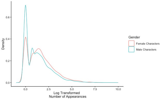
The high appearance record of a small number of male characters is “balanced out” by the low appearance record of a larger number of male characters. Since female characters’ records are more consistent (i.e., the highest performers appear fewer times than the highest performing males), the means of the two groups end up looking almost identical, with female characters taking the lead due to a smaller number of low appearance characters.
The Bottom Line
While there are more male characters in the Marvel universe, X2(1) = 3675.7, p < .001, they do not receive disproportionately more page time than their female counterparts. There are popular male superheroes (e.g., Spider Man, 4043 appearances) and there are also popular female superheroes (e.g., Susan Storm, 1713 appearances). We can’t predict a character’s appearance record from their gender.
Note: the GitHub dataset refers to this variable as “sex”. Sex and gender are different constructs. If you want to learn more about them, the Yale School of Medicine has a great article on their differences and similarities.
When our goal is prediction instead of inference
This is a good reminder of why it’s important to think about data structure and analyses before designing a research experiment. It helps us avoid what Tukey (yes, that Tukey) called a “post-mortem analysis” - instead of analyzing your data to produce valuable insights into a phenomenon, you produce valuable insights about what you should have done differently!
The why is a topic for another post!
Why not BIC values? The size of our sample! The BIC penalizes complex models; since we have 20,000 data points, there’s sufficient statistical power to support the complexity of all three models here.
General linear modeling approaches cannot handle missing values. Removing ALL cases with missing values yields a very different solution, which is why I like to remove missing values on an as-needed basis. Retaining as many cases as possible increases statistical power, while also preserving the representativeness of the sample.
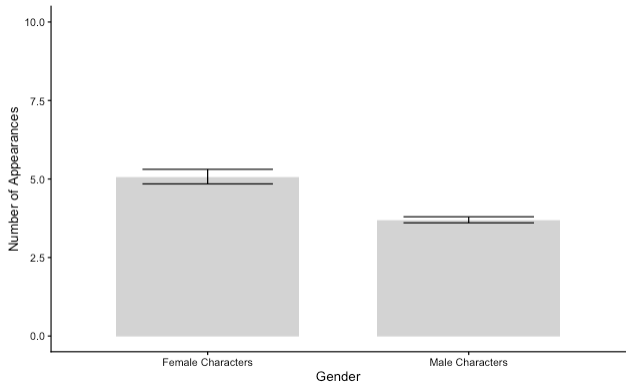
I arrived at this conclusion by back-transforming the estimated marginal means for female (1.62) and male (1.31) characters onto the original scale (5.05 and 3.71, respectively; also illustrated in the figure).
Check out the big brain on Vang! Today I learned about Samuel L. Jackson’s uncredited narrator role in Inglorious Basterds. Begging your pardon for my thinking you’d hidden an enemy of the truth under the floorboards.